Chapter 1 Multiple Linear Regression
In this module we will see how to fit linear regression models. This will serve as a basis for later adjusting models based on other error distributions (Poisson or logistic), focusing also on the spatialization of the results and interact with spatial information.
1.1 Basics of linear regression
Regression is a mathematical method that models the relationship between a dependent variable and a series of independent variables (“Front Matter” 2014). The regression methods allow modeling the relationship between a dependent variable (term \(Yi\)) and a set of explanatory variables that are related to the dependent variable.
In the case of linear regression models, the relationship between the dependent variable and the explanatory variable is linear (thus correctly specified), so that the relation is expressed as a first-order polynomial.
The underlying mathematical procedure is based on the Ordinary Least Squares, so it is common to refer to linear regression using this expression or its English equivalent OLS. In statistics, ordinary least squares (OLS) or linear least squares is a method for estimating the unknown parameters in a linear regression model, with the goal of minimizing the sum of the squares of the differences between the observed responses (values of the variable being predicted) in the given dataset and those predicted by a linear function of a set of explanatory variables. The OLS model can be expressed through the following equation:
\[ Y_i = \beta_0 + \beta_i X_i + \epsilon_i \] Where:
What has to be clear is that we can predict or model the values of a certain variable \(Y_i\) by fitting and applying a mathematical model to \(i\) independent variables of which we know their values.
1.1.1 Assumptions
There are a number of conditions that our data has to meet in order to apply a linear regression model:
Correct specification. The linear functional form is correctly specified.
Strict exogeneity. The errors in the regression should have conditional mean - No linear dependence. The predictors in \(X\) must all be linearly independent (low correlation).
Spherical errors: Homoscedasticity a no autocorrelation in the residuals.
Normality. It is sometimes additionally assumed that the errors have multivariate normal distribution conditional on the regressors.
If you are not familiar with the OLS just keep in mind that we cannot apply the method to any sample of data. Our data has to meet some conditions that we will explore little by little.
1.2 Linear regression in R
Most of the existing regression methods are currently available in R. The calibration of linear regression models with R is possible thanks to the stats package, installed by default in the basic version of R.
For the calibration of linear models either simple (one predictor) or multiple (several predictors) we will use the function lm(). A quick look at the help of the function (help('lm')) will allow us to know how the function works:
lm(formula, data, subset, weights, na.action, method = "qr", model = TRUE, x = FALSE,
   y = FALSE, qr = TRUE, singular.ok = TRUE, contrasts = NULL, offset, ...)
Of all the arguments of the function we are going to focus on the first two (formula and data), since they are the indispensable ones to be able to adjust not just linear regression but any regression or classification model in R. The data argument is used to specify the table (use data.frame object) with the information of our independent variables. Using the formula argument, we specify in the model which of our variables is the dependent variable, and which independent variables in our data.frame object we want to use to carry out the regression. Let’s take a look at the formula first:
v_dep ~ v_indep1 + v_indep2 + . + v_indepn
The formual is composed by two blocks of information separated with the ~ operator. On the left we found the dependent variable specified using its name as it appears on the dataobject. On the right we found the independent variables joined with the + operator. Same as with the dependent one, the independent varibles must be called using their name as it is in data.
We will normally use the above described approach with one exception. Provided we have a data object which only contains a column with our dependent variable and the remaining columns as predictors we can use . after ~ to declare that all the columns in data with the only exception of the dependent variables should be taken as predictors:
v_dep ~ .
The sintax of the formula argument is the same regardless of the kind of regression or classification model we want to use: - Generalized Linear Models - Regression and Classification Trees - Random Forest - Artificial Neural Networks - …
1.2.1 Fitting a linear regression model
Let us now see a simple example of model fitting. We will use the data stored in the file regression.txt that we already used in one of the examples of plot creation. I will import the text file with read.table() and store the data in an object called regression:
Figure 1.1: Structure of the regression.txt file.
- Tavg_max: maximum average temperture in June.
- Tavg: average temperture in June.
- long: longitude in UTM values EPSG:23030.
- lot: latitude in UTM values EPSG:23030.
- d_atl: distance in meters to the Atlantic sea.
- d_medit: distance in meters to the Mediterranean sea.
- elevation: elevation above sea level in meters.
summary(regression)## TavgMAX Tavg long
## Min. :18.20 Min. :13.85 Min. :566050
## 1st Qu.:23.00 1st Qu.:16.80 1st Qu.:628925
## Median :25.05 Median :18.80 Median :690750
## Mean :24.79 Mean :18.64 Mean :687373
## 3rd Qu.:26.90 3rd Qu.:20.55 3rd Qu.:738600
## Max. :30.50 Max. :23.50 Max. :817550
## d_atl d_medit lat
## Min. : 43783 Min. : 670 Min. :4399050
## 1st Qu.:132564 1st Qu.: 92912 1st Qu.:4539325
## Median :211925 Median :159376 Median :4638550
## Mean :216455 Mean :159368 Mean :4615250
## 3rd Qu.:293938 3rd Qu.:227630 3rd Qu.:4700250
## Max. :425054 Max. :325945 Max. :4757850
## elevation
## Min. : 2.0
## 1st Qu.: 302.0
## Median : 505.5
## Mean : 575.7
## 3rd Qu.: 813.8
## Max. :1610.0str(regression)## 'data.frame': 234 obs. of 7 variables:
## $ TavgMAX : num 20.3 23.8 24.4 20.1 20.3 21.9 24.4 20.9 21.2 24 ...
## $ Tavg : num 14.6 16.1 18.1 14.1 13.8 ...
## $ long : int 614350 593950 567250 609150 629450 666750 659450 654050 666850 654150 ...
## $ d_atl : int 305753 271251 279823 319257 306673 317312 335694 347119 359349 369714 ...
## $ d_medit : int 152147 183121 204123 150357 138390 103530 102739 101473 85698 91221 ...
## $ lat : int 4489750 4522150 4512650 4475450 4491350 4489850 4468550 4455350 4446050 4432150 ...
## $ elevation: int 1423 1100 1229 1610 1402 1022 882 828 1308 1186 ...In regression.txt we have all the information necessary to calibrate1 a regression model, that is, variables that can operate as dependent (temperatures) and explanatory variables of the phenomenon to be modeled. Let’s see how to proceed to adjust the regression model and visualize the results. In this example we will use Tavg as the dependent variable and all the other as predictors (except Tavg_max):
lm(Tavg~long+lat+d_atl+d_medit+elevation, data=regression)##
## Call:
## lm(formula = Tavg ~ long + lat + d_atl + d_medit + elevation,
## data = regression)
##
## Coefficients:
## (Intercept) long lat d_atl d_medit
## -4.315e+02 -8.919e-05 1.099e-04 8.516e-05 -6.996e-05
## elevation
## -5.492e-03By executing this instruction we simply obtain the list of regression coefficients resulting from fitting the model. These coefficients give us some information. Strictly the linear regression coefficient gives as the unitary amount of change in the dependent variable on the basis of an increase of 1 of that particular predictor.
However, same as when executing any other function without saving the result, the result is showed in the terminal and lost afterwards. It is appropriate to store the result of the regression model in an object and then apply the summary() function to obtain more detailed results. This is particularly important in this type of functions since the objects generated have much more information than we would simply see in terminal with its execution.
mod.lm<-lm(Tavg~long+lat+d_atl+d_medit+elevation, data=regression)
summary(mod.lm)
##
## Call:
## lm(formula = Tavg ~ long + lat + d_atl + d_medit + elevation,
## data = regression)
##
## Residuals:
## Min 1Q Median 3Q Max
## -4.3020 -0.6010 0.0229 0.5023 2.9665
##
## Coefficients:
## Estimate Std. Error t value Pr(>|t|)
## (Intercept) -4.315e+02 6.269e+01 -6.883 5.61e-11 ***
## long -8.919e-05 1.299e-05 -6.864 6.26e-11 ***
## lat 1.099e-04 1.531e-05 7.179 9.84e-12 ***
## d_atl 8.516e-05 1.139e-05 7.476 1.63e-12 ***
## d_medit -6.996e-05 1.120e-05 -6.245 2.05e-09 ***
## elevation -5.492e-03 2.080e-04 -26.403 < 2e-16 ***
## ---
## Signif. codes: 0 '***' 0.001 '**' 0.01 '*' 0.05 '.' 0.1 ' ' 1
##
## Residual standard error: 0.8881 on 228 degrees of freedom
## Multiple R-squared: 0.8587, Adjusted R-squared: 0.8556
## F-statistic: 277.1 on 5 and 228 DF, p-value: < 2.2e-16Using the function summary(), in addition to the results obtained by calling the object, we obtain additional information such as:
- The significance threshold of the predictors
Pr(>|t|). - The overall error of the model (
residual). - The degree of adjustment of the model (\(R^2\)).
Below we will see a somewhat more detailed explanation of some of the results that will allow us to better understand the results of the model. The coefficients of the predictors and the constant (intercept) are found in Estimates. These are the values we would use in the linear regression formula to obtain the model prediction2. If the a coefficient is positive it means that the higher the value of that variable the higher temperature and vice versa.
The significance thresholds of the explanatory variables determine whether the variables we have used in our model are sufficiently related. We find them in the under the name t value. This value is the Student t test, and is used to determine if a variable is significant, ie if it has relevant influence on the regression model. R automatically sets whether a variable is significant or not through the Signif. Codes. If a variable is found non-significant we should drop it from our model.
The last of the results we will see is the adjustment of the model by means of the coefficient of determination. We will use the Adjusted R-squared value. This value determines the percentage of variance explained by the model. It can be translated, in order to understand it better, as the percentage of success, although it is not exactly that. For practical purposes, the higher this value, the better the model. Their values range from 0 to 1.
1.2.2 Making predictions from our model
Once the model is adjusted, predictions can be made on the value of the dependent variable, as long as we have data from the independent variables. For this, the predict(model, data) function is used. From this function we can not only make predictions from our models but also allow us to carry out their validation.
Let’s look at an example by applying predict() to the data matrix we used to fit the model (regression). We will compare the prediction with the value of the dependent variable (observed or actual data). In this way we can see how similar are the observed values (dependent variable) and the predicted values. However, the ideal is to apply this procedure with a sample of data that has not been used to calibrate the model, and thus to use it as a validation of the results. Generally, a random percentage of data from the total sample is usually reserved to carry out this process. We will do this later.
First we apply predict() and store the result in an object mod.pred. Since this function returns a vector with the predictions, the resulting object will be of type vector:
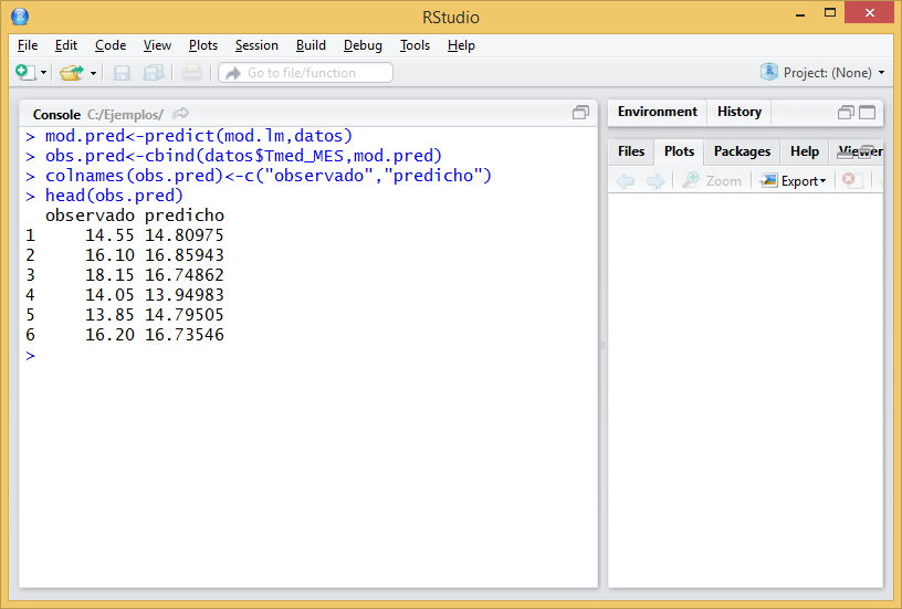
mod.pred<-predict(mod.lm,regression)Then we combine the observed (dependent variable) and predicted data into a new object using cbind(). On the one hand we select the column with the dependent variable in the data object (regression) and on the other the prediction we just made (mod.pred). We save the result to a new object and rename the columns as observed and predicted.
obs.pred<-cbind(regression$Tavg,mod.pred)
colnames(obs.pred)<-c("observed","predicted")
head(obs.pred)
## observed predicted
## 1 14.55 14.80975
## 2 16.10 16.85943
## 3 18.15 16.74862
## 4 14.05 13.94983
## 5 13.85 14.79505
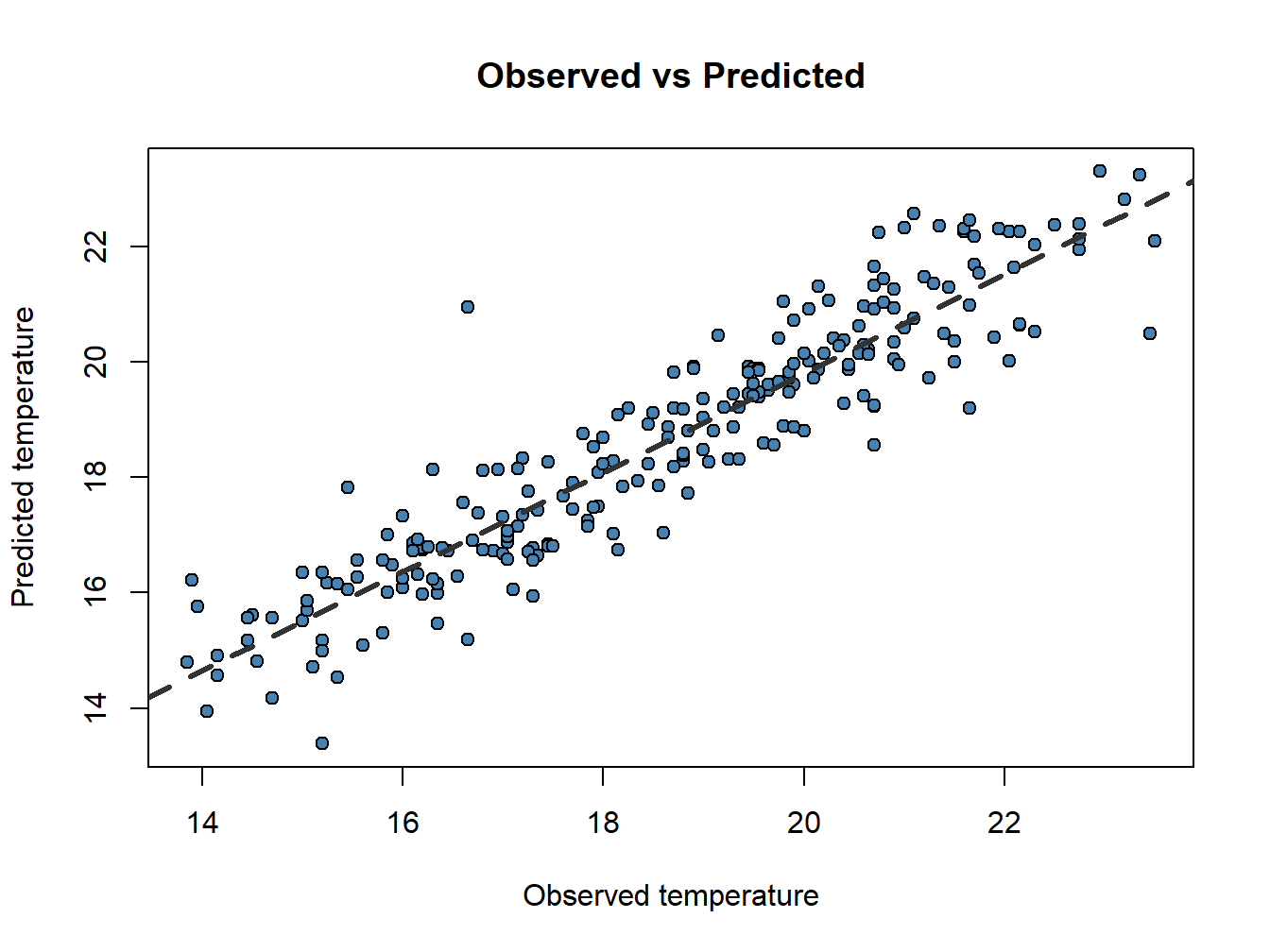
## 6 16.20 16.73546Now, do you remember scatterplots? They are pretty good way to see how well works our model. We can compare the prediction and the actual values like this:
obs.pred<-data.frame(obs.pred)

plot(obs.pred$observed, obs.pred$predicted,
     main='Observed vs Predicted',ylab = 'Predicted temperature', xlab = 'Observed temperature',
     pch=21, col='black', bg='steelblue')
abline(lm(obs.pred$predicted~obs.pred$observed), lty=2, col='gray20',lwd=3)
Now that weird lm() that you already noticed before makes a little more sense. We only can call abline on regression models. Ideally, the perfect fit would display all dots in a 45 degree line starting in (0,0). That would be the \(R^2=1\).
Another thing we can take a look at is the Root Mean Square Error (RMSE). The RMSE is the standard deviation of the residuals (prediction errors3). Residuals are a measure of how far from the regression line data points are; RMSE is a measure of how spread out these residuals are. In other words, it tells you how concentrated the data is around the line of best fit (abline). Root mean square error is commonly used in climatology, forecasting, and regression analysis to verify experimental results. The formula is:
\[ RMSE = \sqrt{\frac{\sum_{i=1}^N (z_{fi} - z_{fo})^2}{N}} \] Where:
- \(z_{fi}\) observed value.
- \(z_{fo}\) predicted value.
- \(N\) is the sample size.
In this case we will create our own R formula obtained from this nice r-bloggers entry:
rmse <- function(error)
{
    sqrt(mean(error^2))
}

rmse(obs.pred$observed - obs.pred$predicted)
## [1] 0.8766348So, taking into account that the RMSE takes the same units that the observed variable, our model predicts temperature with an average error of less than 1 celsius degree.
1.2.3 Collinearity analysis
One of the conditions our data must satisfy is the linear independence of our predictors. This means that our explanatory variables must be independent one another or what is the same, have low correlation values.
Correlation is a measure of the degree of association between to numeric variables. There are several methods to measure correlation both parametric (at least one variable must be normally distributed) and non-parametric (no assumptions in the data).
- Parametric: Pearson correlation coefficient.
- Non-parametric: Spearman’s \(\rho\) and Kendall’s \(\tau\) rank correlation coefficients.
Regardless of the method, R uses the function cor() to calculate a coefficient of correlation. By defautl Pearson's R is calculated although the method argument allows to change the method to a non-parametric alternative.
cor(regression)## TavgMAX Tavg long d_atl
## TavgMAX 1.0000000 0.9384827 0.4416862 0.27237366
## Tavg 0.9384827 1.0000000 0.4018594 0.29814899
## long 0.4416862 0.4018594 1.0000000 0.57574513
## d_atl 0.2723737 0.2981490 0.5757451 1.00000000
## d_medit -0.4015863 -0.4287400 -0.7589245 -0.95258210
## lat -0.1667702 -0.2259106 -0.2921629 -0.94604910
## elevation -0.7789850 -0.8629255 -0.2375738 -0.01776881
## d_medit lat elevation
## TavgMAX -0.4015863 -0.16677016 -0.77898498
## Tavg -0.4287400 -0.22591063 -0.86292553
## long -0.7589245 -0.29216294 -0.23757377
## d_atl -0.9525821 -0.94604910 -0.01776881
## d_medit 1.0000000 0.83632353 0.17570069
## lat 0.8363235 1.00000000 -0.02359441
## elevation 0.1757007 -0.02359441 1.00000000cor(regression,method = 'spearman')## TavgMAX Tavg long d_atl
## TavgMAX 1.0000000 0.9430791 0.4582967 0.29512643
## Tavg 0.9430791 1.0000000 0.4139180 0.30806962
## long 0.4582967 0.4139180 1.0000000 0.58866202
## d_atl 0.2951264 0.3080696 0.5886620 1.00000000
## d_medit -0.4244320 -0.4375261 -0.7589619 -0.95404315
## lat -0.2627180 -0.3056250 -0.3180236 -0.93905906
## elevation -0.8044907 -0.8849362 -0.2816401 -0.09692695
## d_medit lat elevation
## TavgMAX -0.4244320 -0.2627180 -0.80449069
## Tavg -0.4375261 -0.3056250 -0.88493622
## long -0.7589619 -0.3180236 -0.28164007
## d_atl -0.9540432 -0.9390591 -0.09692695
## d_medit 1.0000000 0.8499073 0.24769852
## lat 0.8499073 1.0000000 0.11658310
## elevation 0.2476985 0.1165831 1.00000000Any correlation coefficient ranges from -1, indicating high inverese correlation4, to 1, indicating positive correlation. Values around 0 indicate no correlation.
Ideally, our predictors must be uncorrelated. Therefore, correlation values between -0.4 to 0.4 are rather acceptable. If correlation is higher we must drop one of those predictors from our regression model.
1.2.4 Scripting our model
The usual thing is to create small scripts joining the necessary instructions to build a model that solves a specific problem. Both the standard R interface in Windows and RStudio provide interfaces for script development. If you work in terminal cmd you will have to use a text editor with ability to interpret code (Notepad++ for example). In RStudio we simply press the button under File (Figure 1.2) to access the scripting window and we will choose the option R Script:

Figure 1.2: Open script button
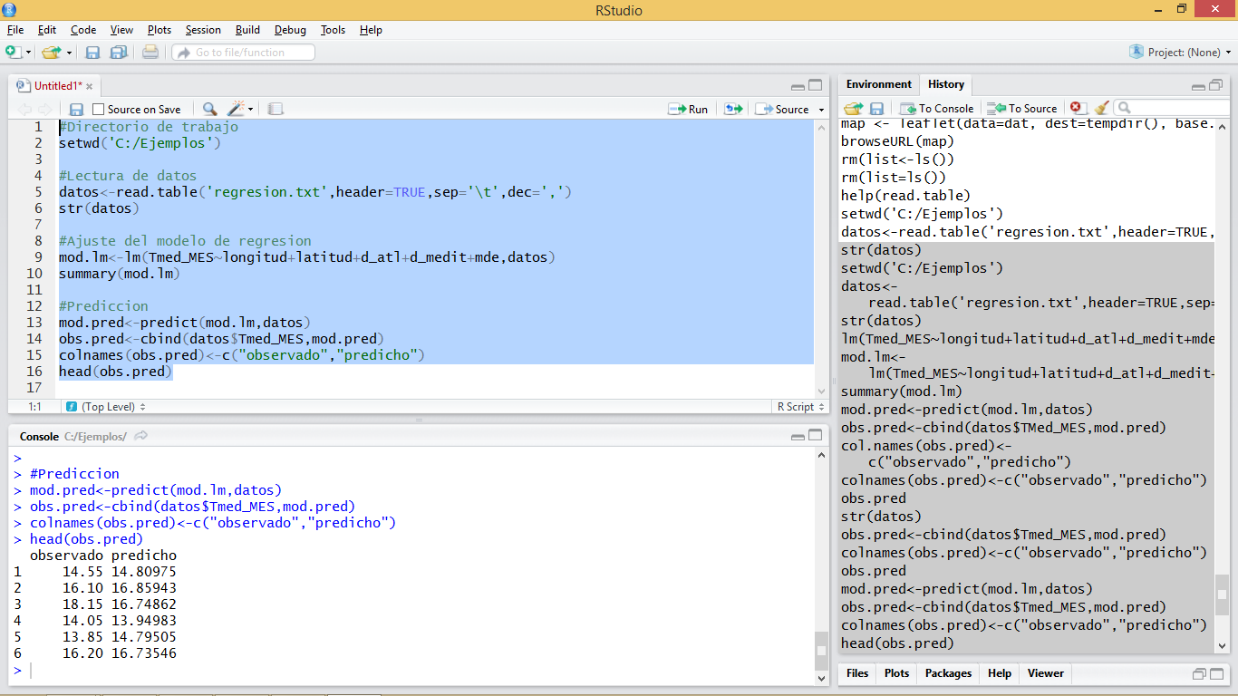
Once this is done, just write the instructions that you want to execute in the appropriate order. Then select them and press the Run button (the green one like a Play button). In the following screenshot (Figure 1.3) you can see an example where you have entered the instructions to carry out the regression model that we just created5.

Figure 1.3: Scripting window example
1.3 Considerations for further developments
So far what we have done is simply to model the relationship between a dependent variable (mean temperature) and a series of explanatory variables. We have seen that we can make “predictions” from the adjusted models. This implies that if we had spatially distributed information about the explanatory variables (raster layers for example) we could generate maps of mean temperature values from the regression model. Later we will see how to do this hand in hand with some packages for manipulation of spatial information.
References
“Front Matter.” 2014. In Applied Regression Analysis, i–xix. John Wiley & Sons, Ltd. doi:10.1002/9781118625590.fmatter.